Бесплатный фрагмент - Jump into Excel. Training Course from Beginner to Intermediate in two hours

Briefly about this course and me.

This Training Course is designed for two hours. Information about my video course «Jump into Excel. From Beginner to Intermediate in two hours», test tasks and files with examples of the use of basic Excel functions can be found on my website (find them at the end of the book).

Knowledge from the Course will be enough to perform all tasks within the work functionality for most employees. The course is a step-by-step instruction from scratch. Accompanied by screenshots with explanations. From scattered and incomplete source information, we gradually create and prepare for printing a final table with the processed data. In the course of the action, we get acquainted with Excel and focus on the most frequently used features of the program for data processing and visual presentation of results, learn to work with the main functions.

The course will be useful to anyone who wants to learn how to work with this magical program. Excel allows you to find and extract numbers and text from separate source files, make almost any calculations, and transform the source data according to your request. In Excel, you can save the final result in any form: from plain text and tables to pivot tables and graphs. In contrast to complex and expensive special programs, the settings of which can only be worked with by experienced programmers, Excel is intuitive, easy to edit, and accessible to everyone. Therefore, Excel is widespread and its knowledge at an intermediate level is mandatory for applicants for high-paying positions in almost all areas of business.

I have met students who, after completing many hours of Excel courses, experienced difficulties in elementary functionality. Many have tried unsuccessfully to read and memorize multi-page detailed books on the vast possibilities of Excel, and now after that they believe that learning Excel too complicated and too time-consuming. I dare to give you a piece of advice: don’t be afraid to start studying, you can learn the essentials in two hours. And if you suddenly have a specific task that requires additional knowledge, you can easily and quickly find it by searching on the Internet or using the help inside the program. Do not waste your time on many hours of courses and loading your brain with unique knowledge that is not necessary in practice. Bravely jump into Excel and start solving specific practical problems of your business faster with its help, rather than out-of-touch tasks for knowledge of rarely used Excel functions. And only when you find out that your knowledge is not enough for your work, only then delve into the specific issue that you want to understand better.

Why spend money on this course when you can learn everything on the Internet?

Yes, you can learn on your own, but it will take more time. And the cost of this time spent by you will be many times more than the cost of this course. By purchasing this course, you end up saving money. In addition, there are many features in Excel that are rarely used in practice. If you study everything, there is a risk of missing the main thing, overloading the brain with the secondary.

Who are you and why should I choose your course?

My name is Skorodumov Aleksey, I live and work in St. Petersburg, I have a PhD in economics. For many years I have been working with Excel continuously, having completed hundreds of orders for both large and small companies from various business areas with its help. My Course is good because it allows you to learn in a short time the most important things in Excel, which are really used in practice.

You can contact me for possible cooperation through my website or by mail (find them at the end of the book).

---

Creating an Excel file from scratch

Let’s begin.

Imagine that a beginner who is completely unfamiliar with Excel is assigned a task: to prepare an Excel file with information about company’s employees.

At the same time, you need to use data both from the HR department and the secretary, and then save them on different sheets.

The final file should be a report table for printing with the following columns: Department, Position, Surname, First Name, Patronymic, Date of employment, Date of birth, Experience of full years on the date of the report, Age of full years on the date of the report. The table should be sorted by the employee’s surname.

So, let’s figure out step by step how to complete this Task.

To begin with, let’s choose a place or «Folder» on the computer where the Excel file we created will be stored, and also choose a name for them. For example, let’s create a «Task» folder on the Desktop, and in it we will create an Excel file with the name «Employees».

Note for beginners: if the desktop on the computer is not visible at the moment of work, for example, due to the fact that the screen is completely occupied by an open application, we will first open access to the desktop, and «minimize» all open windows of other applications. If we do not see the «Minimize all windows» button (its display depends on the computer settings) then hover the mouse cursor over the lowest part of the screen, a strip called the «Taskbar». Then right-click, and in the menu window that appears, left-click on «Show the desktop».

All other windows with open applications will minimize and the Desktop will open to us.

So, let’s create a new folder.

Hover the mouse cursor over any free space on the Desktop and click the right mouse button. In the menu window that appears, hover the mouse cursor over «New», then hover over the «Folder» and click on the left mouse button.

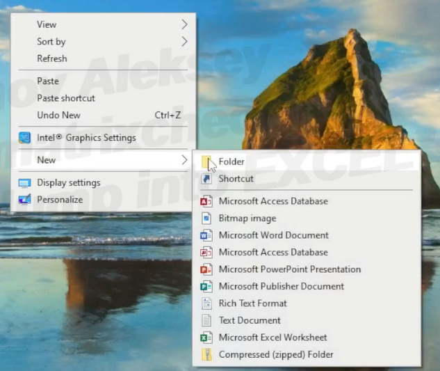
A folder with the highlighted name «New folder» appeared.

At the moment of selecting the text in the folder, we change its current name «New folder» to our name «Task» by typing the text from the keyboard and pressing the «Enter» key.

If we later want to rename the «Task» folder to any other name, hover the mouse cursor over this folder and click the right mouse button, select «Rename»

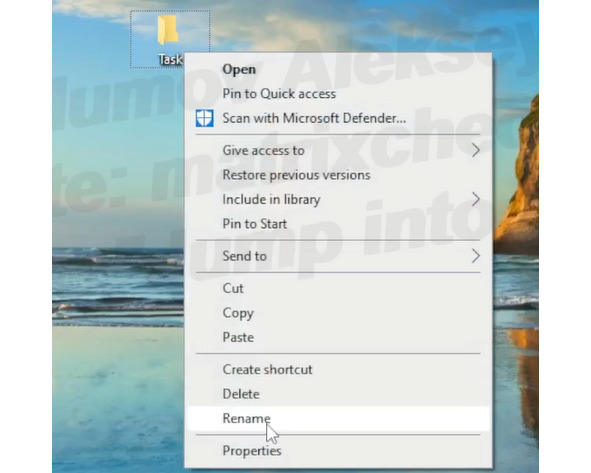
and type in the name we want,

for example, «Folder». Then you can press «Enter».

Return the name «Task» to the folder.

Now, open the created folder «Task».

To do this, hover the mouse cursor over the «Task» folder and click the right mouse button. In the menu window that appears, hover the cursor over «Open» and click on the left mouse button.

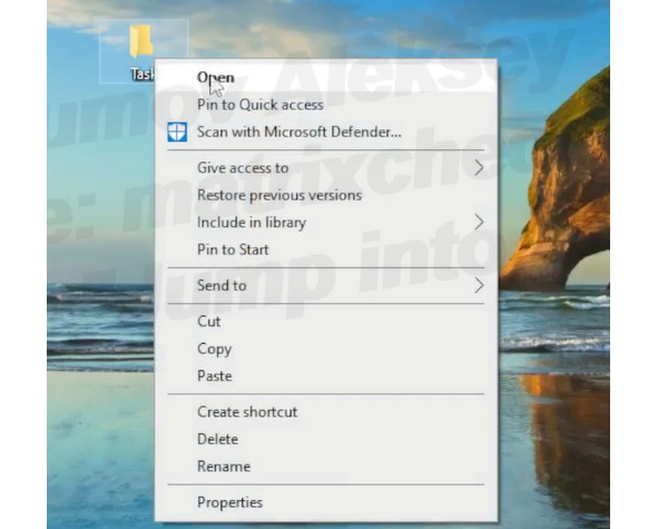
An empty folder opens. Let’s create a Microsoft Excel file in it.

To do this, hover the mouse cursor over any free space in the open folder «Task» and click the right mouse button. In the menu window, select «New», and in the next menu window that opens, select «Microsoft Excel Worksheet».

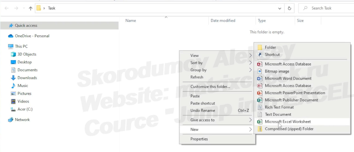
The file «Microsoft Excel Worksheet» appeared. We can straightaway rename it to our name «Employees». So, type in «Employees» from the keyboard, and press the «Enter» key on the keyboard.

In the same folder, we will copy the files with the initial information received from the HR department and from the secretary.

Let’s say these files were transferred to us on a flash drive or saved in a shared folder.

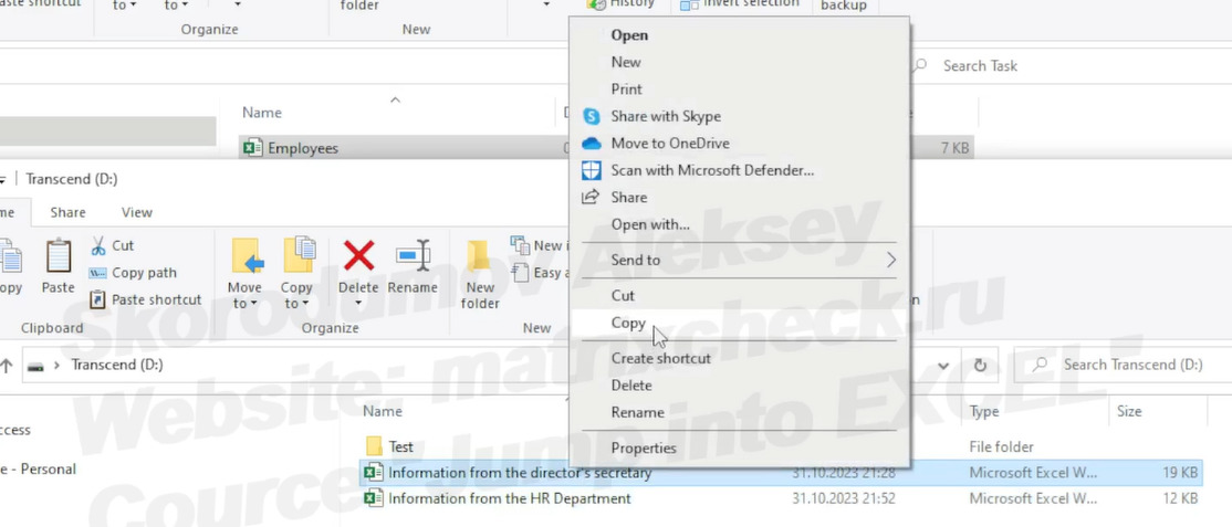
To copy files to the «Task» folder, first open a flash drive or a shared folder. In our case, this is a Transcend flash drive. In the folder that opens, right-click on the desired file and select «Copy».

Then go to our «Task» folder, right-click and select «Paste».

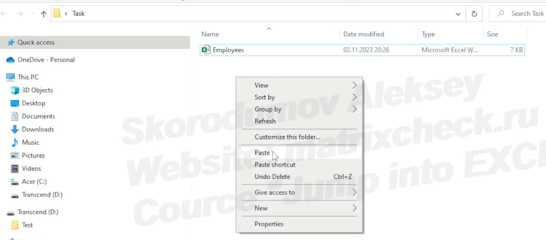
Now we can see the file appeared. We will do the same with the second file. First copy and then paste it. Now all three files are in our «Task» folder: two with the initial information, and the third file created by us, «Employees», in which we will prepare the Results.

Now let’s start filling out the created «Employees» file with information.

We can open the file «Employees» as we opened the folder: hover the mouse cursor, click the right mouse button and select «Open» from the menu. Or we can do it in another way: hover the mouse cursor over the file and double-click with the left mouse button. The file opens.

Introduction to the Interface

The Excel file will open as a blank sheet looking like this. The specific view depends on the computer settings and the version of Excel.

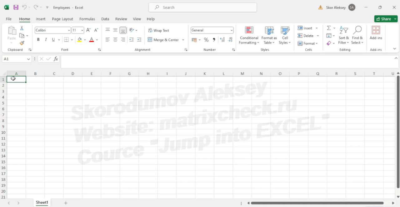
Let’s get acquainted with what we see.

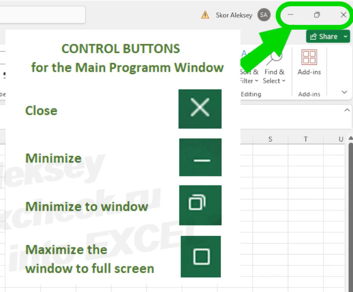
Control buttons for the main program window

They are located in the upper right area of the Excel window. They allow you to close a file, Minimize it, minimize it into a window, expand the window to full screen.

The Quick Access Toolbar is located in the upper left area of the Excel window.

If we often use the same commands, we can bring the command buttons here and run commands from here. For example, the «Save changes» command is often used. If you do not click it, then everything you have done in the file after opening it will disappear after closing the file. The «Undo last action» command is also often used. For example, if you accidentally deleted a column with the necessary information, clicking on this command will return you to the state that was before the deletion.

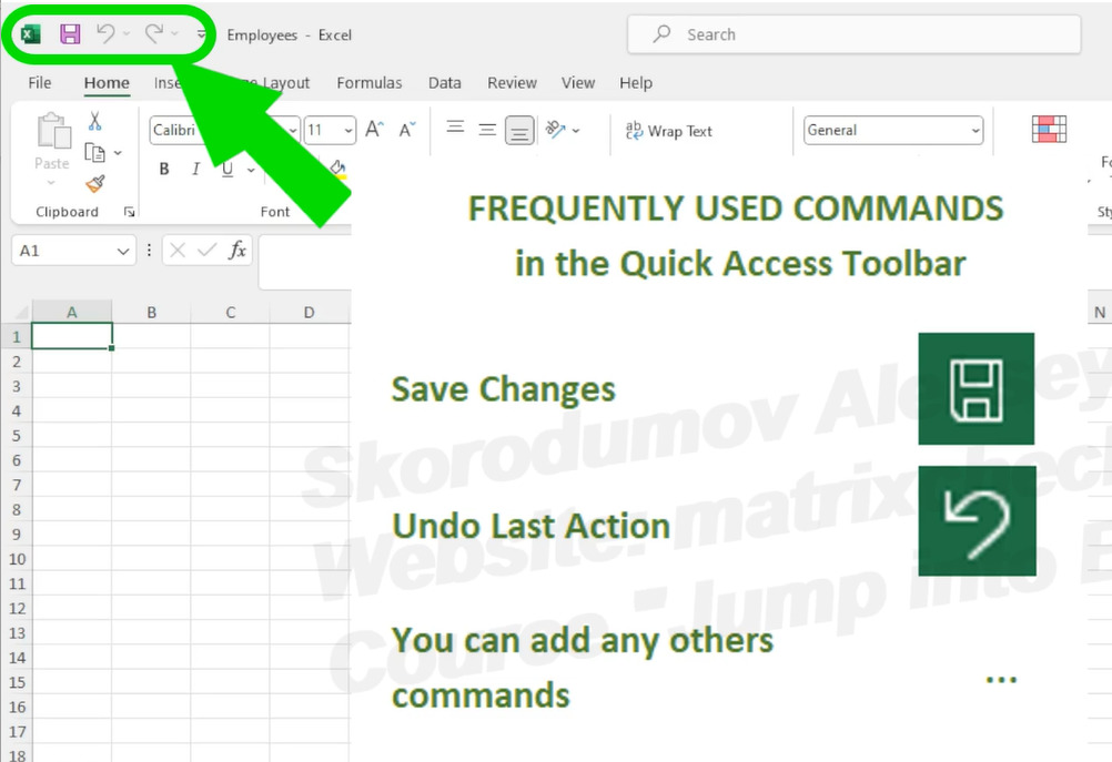
If desired, we can add any other commands to the Quick Access Toolbar by clicking on the edit button of the Quick Access Toolbar. Select «More Commands»

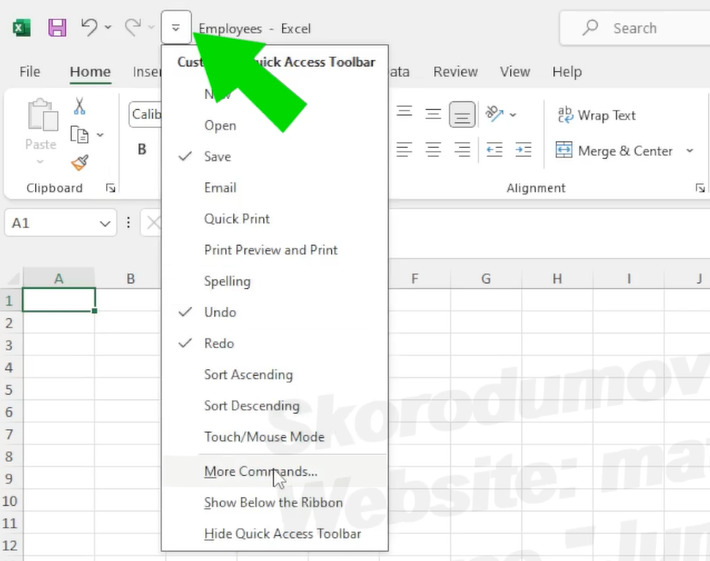
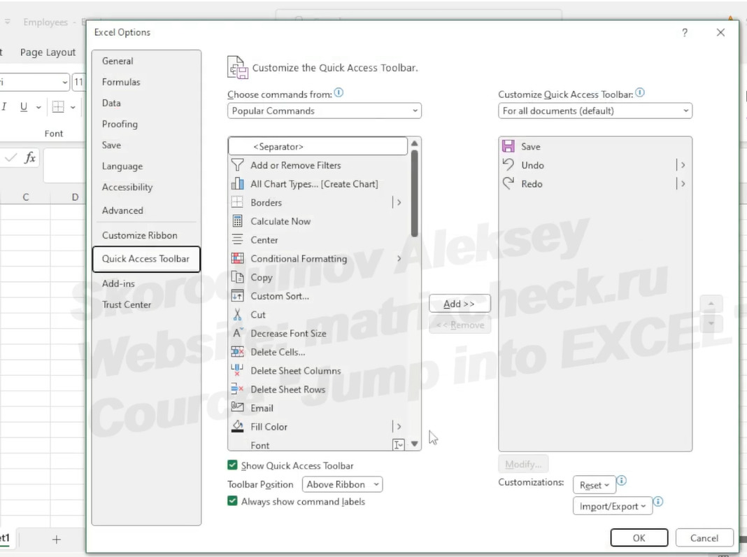
and add the necessary ones.

Tabs.

Under the quick access toolbar there is a ribbon with available tabs: Home, Insert, Page Layout, Formulas, Data, Review, View. As you can see, each tab has its own set of commands.

This set of commands can be edited if desired — you can add or remove commands. I do not recommend beginners to engage in such editing — everything you need is already configured by default. But if we really need to add our own commands, then it’s easy to do: hover the mouse cursor over any point of the tabs, click the right mouse button, select «Customize the Ribbon» and get to the tab editing menu, where we can not only add any command to any tab, but also create our own tab.

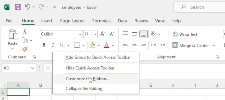
For example, select «New Tab»,

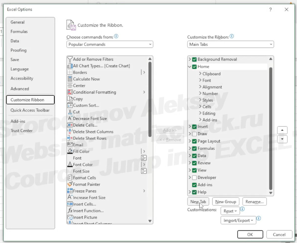
name it «Aleksey» (it’s my name),

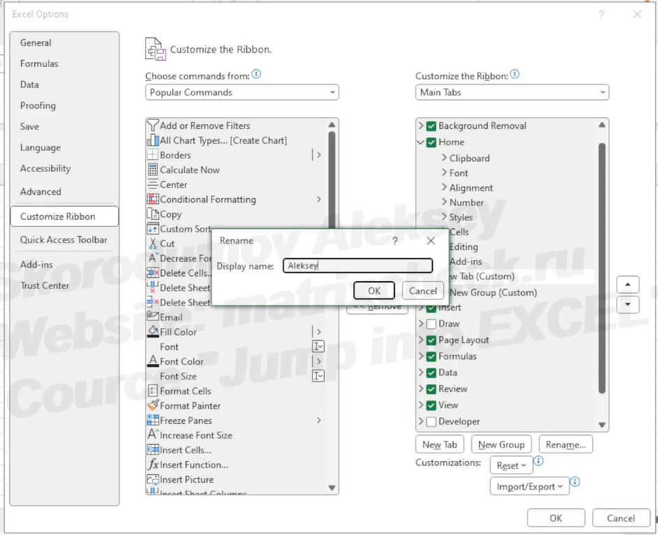
and we can add any commands to this tab. Click «OK».

Now, we have a new tab with the name «Aleksey».

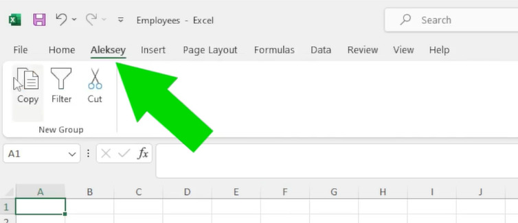
Since we don’t actually need this tab, we Remove it.

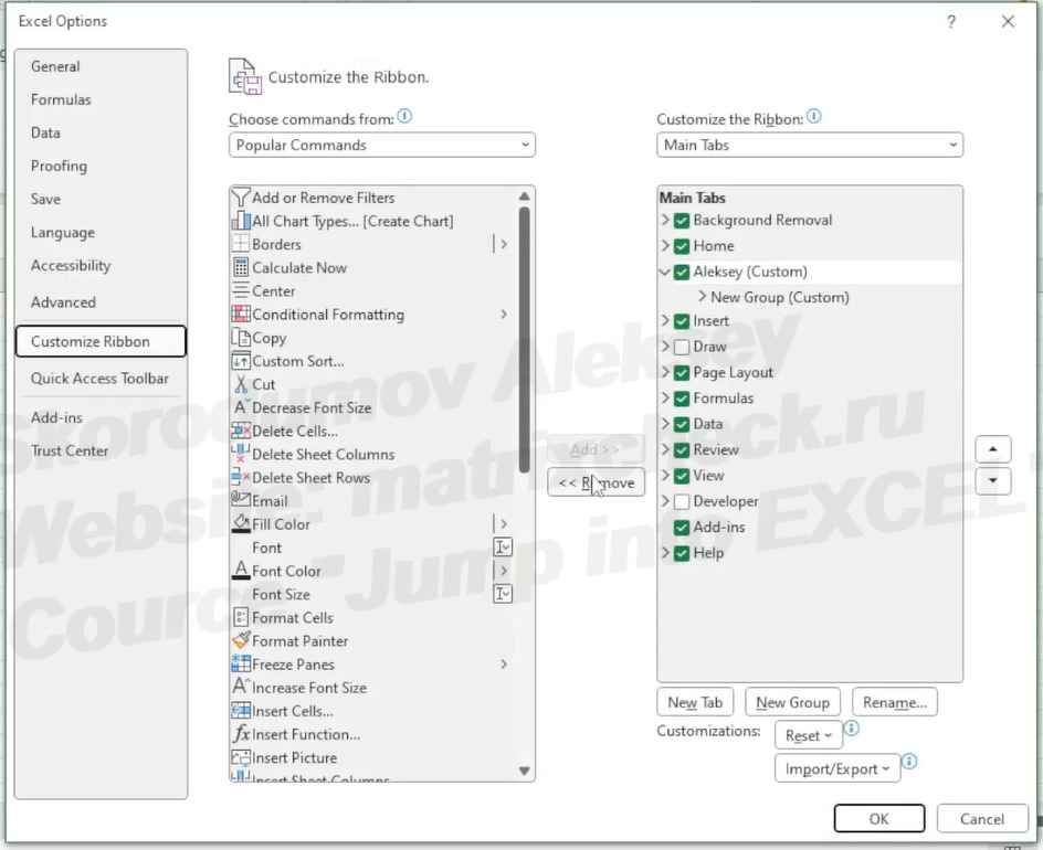
And it disappeared.

Tab commands are located under the ribbon with the tabs. When opening a file, we see the commands of the «Home» tab, since the «Home» tab opens by default. If we move to another tab, for example, the «Formulas», then we will see the commands of this other tab.

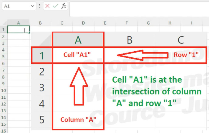
To access individual cells inside a spreadsheet, the Cell names are used. The Cell name is a combination of its column (denoted by the Latin letter A, B, C, D …) and its row number (1, 2, 3, 4, 5 …). In total, there are more than 16,000 columns and more than a million rows in the Excel file on one sheet, that is, more than 16 billion cells on each sheet.

Object name field.

By default, there we see the name of the active cell in which the table cursor is located therefore, the active cell is often called «Highlighted». We can select any object: a cell, a group of cells, a table, a graph and assign (by typing) any name in this field of the object name, for example «Table1», in order to further refer to the named object by its specific name.

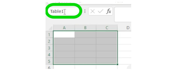
In practice, this feature is often used when working with a lot of arrays and in long formulas to shorten them. In other cases, it is not recommended to specify the names of objects without a necessity.

The Function Wizard button is used for quick search and insertion into the active cell of any of the built-in Excel functions. We will get acquainted with the basic built-in Excel functions later.

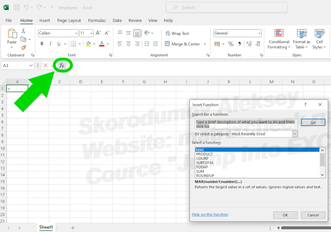
The Formula bar shows the contents of the Active Cell. If the active cell contains a constant, then both in the cell and in the formula bar we will see this constant, for example «2». But if the active cell contains a formula, for example "=2+2», then in the formula bar we will see the formula itself, and in the cell, we will see the result of the formula — «4». The text of the formula contained in the cell can be edited.

The labels with the Names of the sheets are at the very bottom of the window. Sheets can be renamed, added, deleted, renamed again.

There can be hundreds of sheets in a single Excel file. But in practice, they are usually limited to 10, maximum 20 sheets. The thing is that when there are a lot of sheets, it becomes inconvenient to search for information.

Scrollbars allow you to see adjacent areas of the sheet that are not currently visible. The row scroll bar is on the right, and the column scroll bar is at the bottom of the sheet. We hover the mouse cursor over the viewing direction, click the left mouse button and do not let go until we find ourselves in the place that we are interested in seeing. If we scroll through several rows or columns, we stop seeing the active cell, but at the same time, we will still see which cell is active in the object name field.

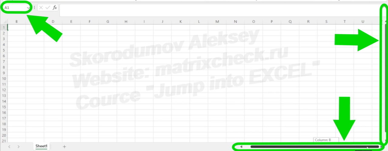
Please note: the active cell itself does not shift at the same time. It’s still A1.

To make another cell active, use the mouse or keyboard arrows instead of scroll bars. To select another cell with the mouse, just hover the mouse cursor over another cell, for example D1, and click the left mouse button.

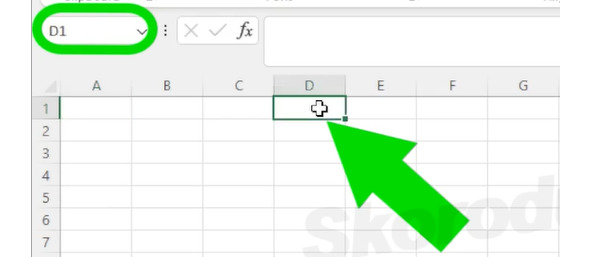
You can also move the active cell using the arrows on the keyboard, which are located in the lower right corner of the keyboard.

Filling in the file with the initial information

Now let’s go back to our task and start filling in the file with the initial information.

Let’s open the first of the sent files «Information from the director’s secretary».

As you can see, there is not complete information on the task: there is no Date of birth, no Date of employment, no Experience years and Age. But at the same time, there is information that was not required by the assignment: a Work phone and an E-mail.

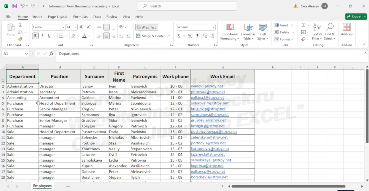
We will copy all this information into our «Employees» file on a separate sheet, which we will call «Information from secretary».

In order to rename «Sheet1» to the name «Information from secretary», hover the mouse cursor over «Sheet1», press the right mouse button, select «Rename» and type in «Information from secretary», then press the «Enter» key.

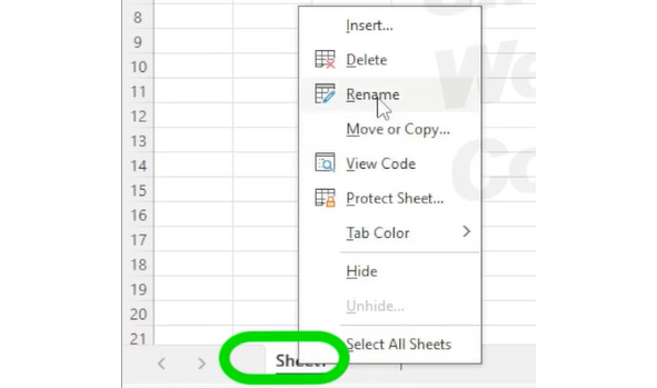
and type in «Information from secretary», then press the «Enter» key.

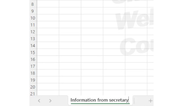
Copy operation

Before copying, it is necessary to highlight the cell that we are going to copy. «Highlight» means to stand on a cell with a tabular cursor. This can be done using the arrows located on the keyboard in the lower right corner.

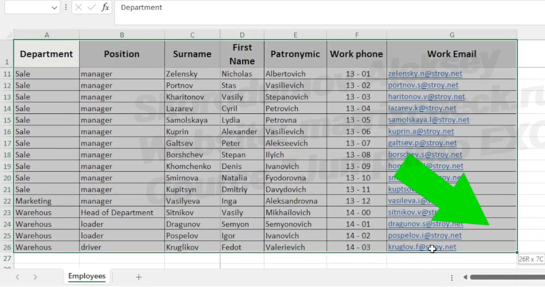
You can also select a cell using the mouse cursor. Hover the mouse cursor, for example, on the cell «G26» and click the left mouse button. To highlight the entire copied range, we stand on its corner cell, for example «G26». Click on the left mouse button and, without releasing this button, drag the cursor to the opposite corner. And only after bringing it to the end — we release the left mouse button pressed.

Thus, the entire block of cells is highlighted.

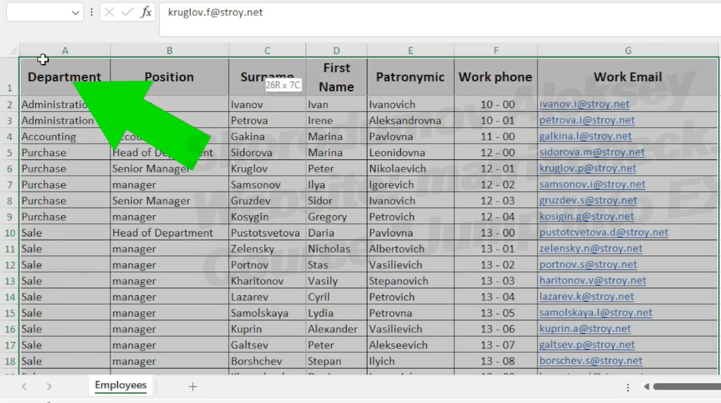
Let’s repeat it again. We stand on the cell «A1», press the left mouse button and drag the cursor now to the lower opposite corner. When dragged — release the left mouse button.

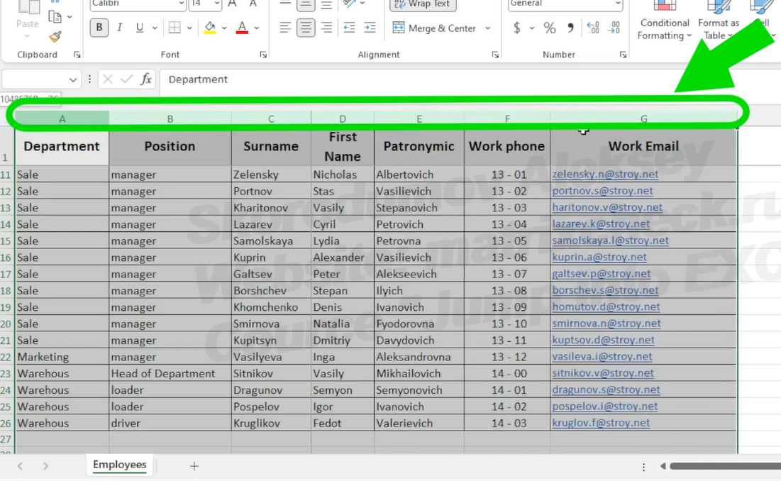
There is another way to select the desired cells. We can select for copying. Not only the range A1:G26, which is a part of the columns A:G, that is, but all the cells of the columns A:G at once. To do this, hover the cursor over the name of column «A», above cell A1, click on the left mouse button and, without releasing it, drag the mouse cursor to the right until column G is highlighted. Release the pressed left mouse button.

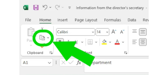
After the range for copying is selected, click on the «Copy» button located on the «Home» tab.

Instead of using the «Copy» button, we can hover the mouse cursor over the selected range, right-click and select «Copy».

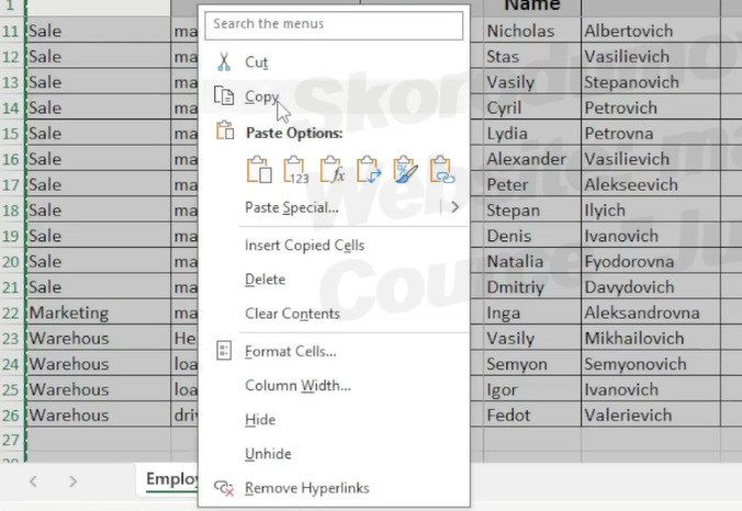
For copying, the «Ctrl» and «C» keys located on the keyboard are also often used. First, press the «Ctrl» and, without releasing it, press the «C» key with the second finger.

Regardless of the chosen copying method, the result will be the same: a copy of the selected fragment gets to the Clipboard and is ready for insertion in any other place, both in this file and in any other file. Around the copied fragment, a temporary dynamic dotted line appears, indicating copies of which cells are currently in the Clipboard.

Paste operation

We stand with the tabular cursor on the cell in which we are going to insert the data on our «Information from secretary» sheet.

Since we are going to insert not one cell, but a whole array of data, we must stand on the upper left cell of this array (in this case it is cell «A1»), below which and to the right of which the entire array will be inserted.

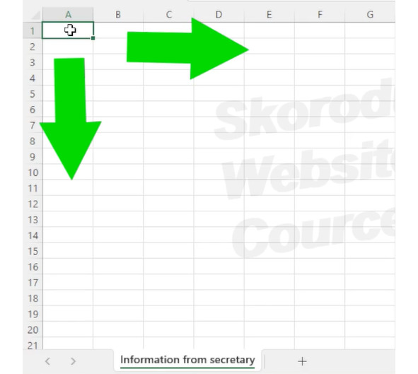
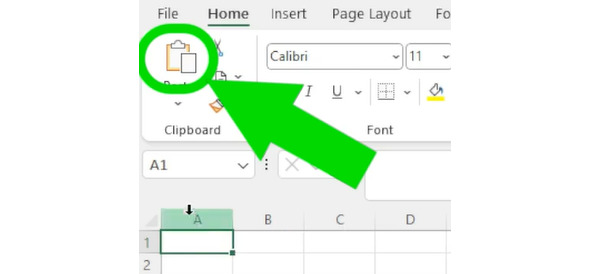
Click on the «Paste» button located on the «Home» tab.

Instead of the «Paste» button, you can use the keyboard shortcut «Ctrl» and «V». You can also hover the mouse cursor, right-click and select «Paste».

In the data copied to the «Information from secretary» sheet, not all words are fully readable, since the column width is less than the width of some words.

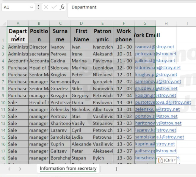
If we want to align column A by width, that is, to make the width of column «A» such that the longest word in column «A» is visible, then hover the mouse cursor over the right border of column «A» and double-click with the left mouse button.

If we want to align several columns in a similar way, then select these columns from «A» to «G», hover the mouse cursor over the border of any two of them, for example between «A» and «B», and double-click the left mouse button with a small interval. All columns have «moved apart».

To quickly select all columns and all rows of the entire sheet at once, use a left mouse click on the upper left corner area located to the left of column «A» and above row «1». This method of selecting the entire sheet is used not only when adjusting columns or rows in width, but also when quickly copying the contents of the entire sheet at once.

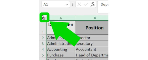
Thus, we copied, pasted, and aligned the width of the inserted array of initial data.

Now we will copy the data from the second file with the initial data «Information from the HR Department» to a sheet, which we will call «Information from HR». Since we don’t have a second sheet in the file yet, we need to create it. We will do this by hovering the mouse cursor over the name of the sheet, similar to how we did when renaming the sheet, and click the right mouse button. Only now we will choose not «Rename», but «Insert», and then select «Worksheet». Click «Ok».

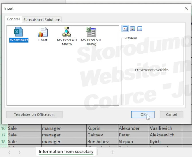
Rename this new «Sheet1» to «Information from HR», copy the information from the HR department to it, similar to how we did it with the information from the secretary.

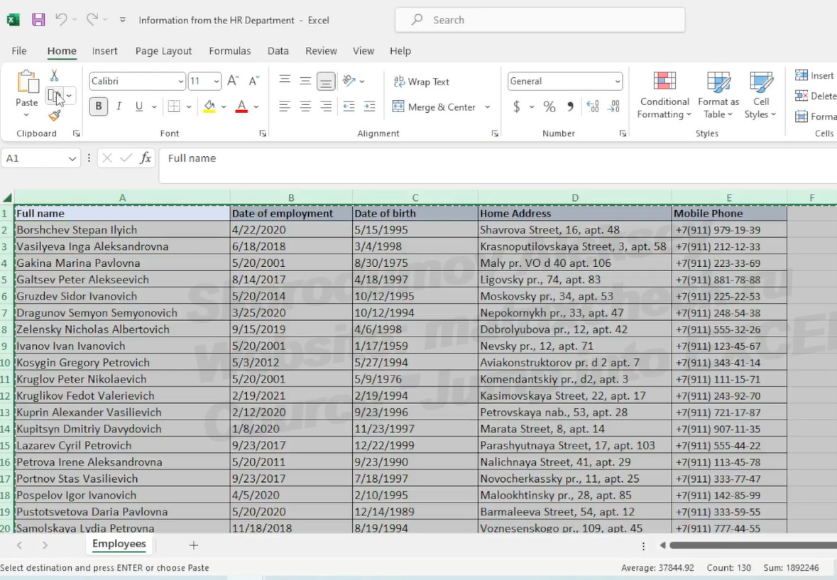
Since this time, we copied and pasted all the rows and all the columns of the sheet at once, we did not have to additionally align the columns in width.

Let’s create another, third sheet, which we will call «Result». On which we will enter information from both the «Information from HR» sheet and the «Information from secretary» sheet.

Please note: the active sheet is highlighted with a white fill. To move to another sheet, hover the mouse cursor over it and click the left button.

Now, let’s move to another sheet. And let’s go to the «Result» sheet again. The layout of the sheet can also be changed. To do this, hover the mouse cursor over the name of the sheet, right-click, select «Move» or «Copy» and, for example, move to the end.

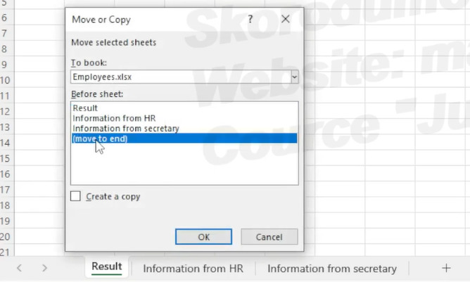
Editing tables

We proceed to fill out the «Result» sheet.

First, copy the information from the sheet from the Secretary to the «Result» sheet. Select and copy columns A:E with the names Department, Position, Surname, First Name, Patronymic.

Copied.

As it often happens in practice, we are faced with a small problem: the names in the file that was provided to us from one source (from the Secretary) are arranged in a different order. The rows are sorted differently than the rows with surnames in the file that we received from another source (HR department). If the rows with surnames on both source sheets (both from the Secretary and from the HR Department) would have the same order, then copying would be simple. We would select the columns we need (with dates of birth and employment), copy them and paste them. But in our case, this cannot be done, because it will lead to an error — in the file from the HR Department and on the sheet «Information from HR» in the second row is the surname «Borshchev», while in the file from the Secretary and on the sheet «Result» the second row is occupied by «Ivanov».

If we just copy and paste the columns from the «Information from HR» sheet to the «Result» sheet with data, as on the «Information from Secretary» sheet, then the second row with Borshchev’s Date of birth and Date of employment will be substituted into the second row with Ivanov’s Department, Position, Surname, First Name and Patronymic.

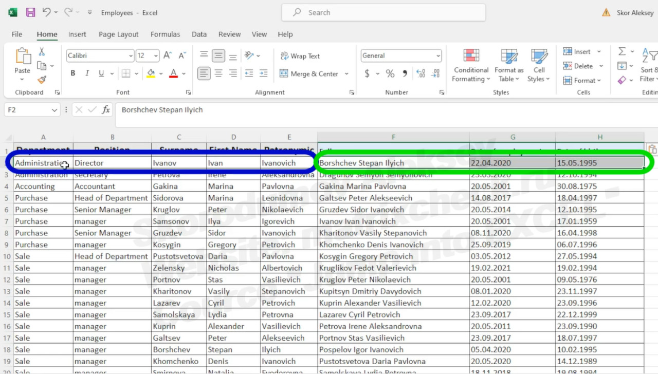
To avoid this error, we will perform preliminary data processing — we will put the rows on the «Result» sheet in the same alphabetical order as they are sorted on the «Information from HR» sheet. So that the line with the surname «Borshchev» on the «Result» sheet would become the second, immediately under the header, as well as on the «Information from HR» sheet. After that, we will be able to copy the columns from the «Information from HR» sheet to the «Result» sheet, and Borshchev’s data will be copied to the row with Borshchev, and not with Ivanov.

Let’s use Sorting for this.

Sort operation

Select the area for sorting (columns A:E or cells A1:E26), click on the «Sort» button on the «Data» tab, select «Sort by…", «Surname», in the window that appears, select the alphabetical sorting order «From A to Z», and click «Ok».

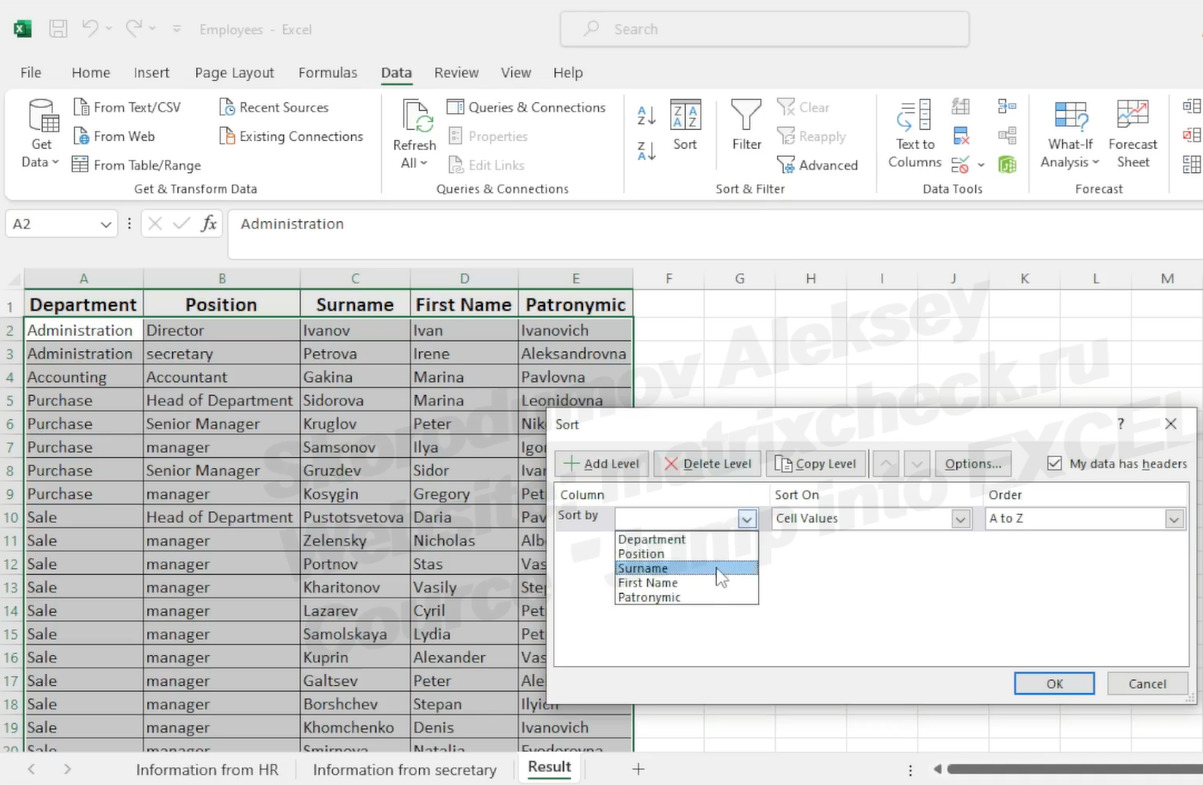
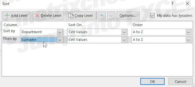
Please note: If we wanted to sort the names of Departments in alphabetical order, and then within these departments by Surname, we would first select «Sort by — Department», and then add a second level of sorting by clicking on «Add Level» in the upper left corner of the menu, and in the second level that appeared we would select «Surname».

After the sorting is done, the order of the rows with surnames on the «Result» sheet matches the order of the rows on the «Information from HR» sheet.

Note: Sorting (and much more) can also be done using the menu that appears when you right-click. Using the right mouse button to open the menu is a very useful skill that speeds up your work in Excel.

Copy the data from the «Information from HR» sheet to transfer to the «Result» sheet.

Select three columns on the «Information from HR» sheet: «Full name», «Date of employment» and «Date of birth». We don’t need the Full name column for the task, but we use it to make sure that the rows with the surnames of employees after sorting now match everywhere.

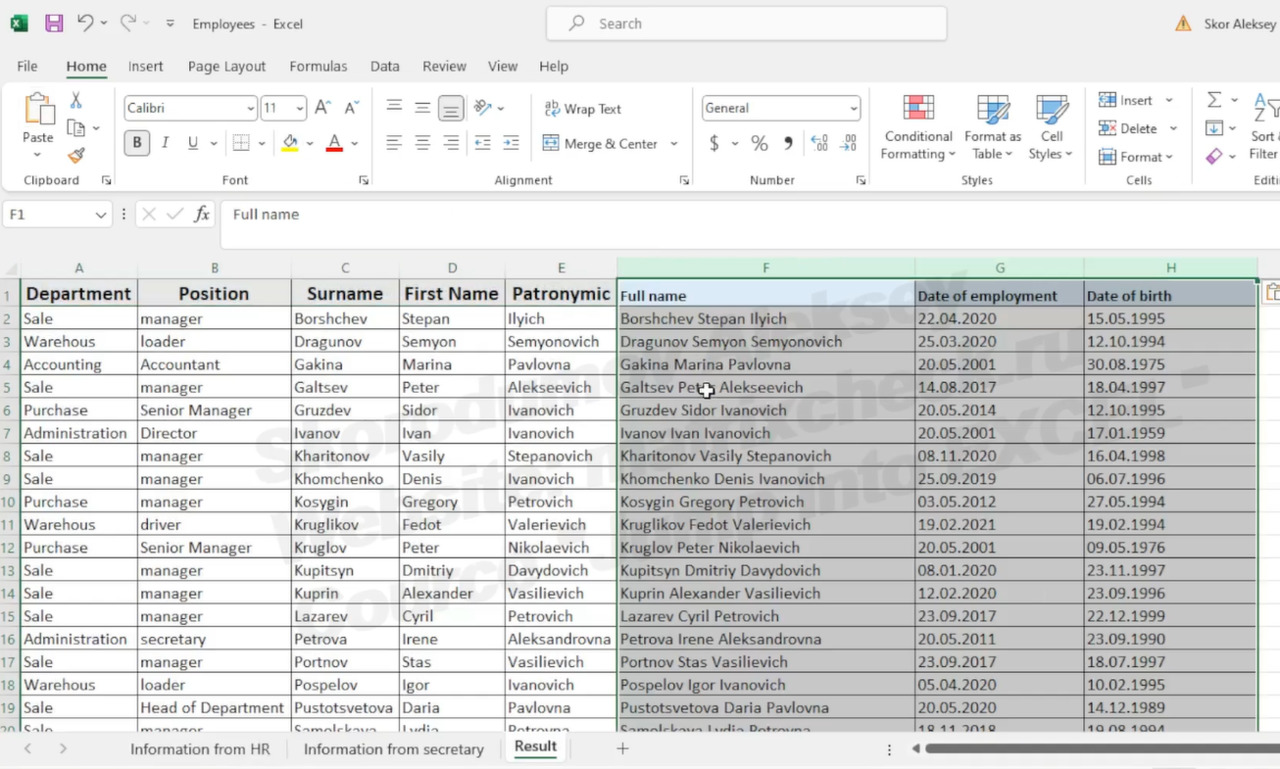
After visual verification that the order of the rows is correct (that is, the last name from column «F» with the full name coincided with the last name from column «C»), the extra column «F» with the Full name must be deleted.

Deleting a column

Select column F by hovering the mouse cursor over the heading F and click the left mouse button. Then click on the right mouse button. In the menu that appears, select «Delete».

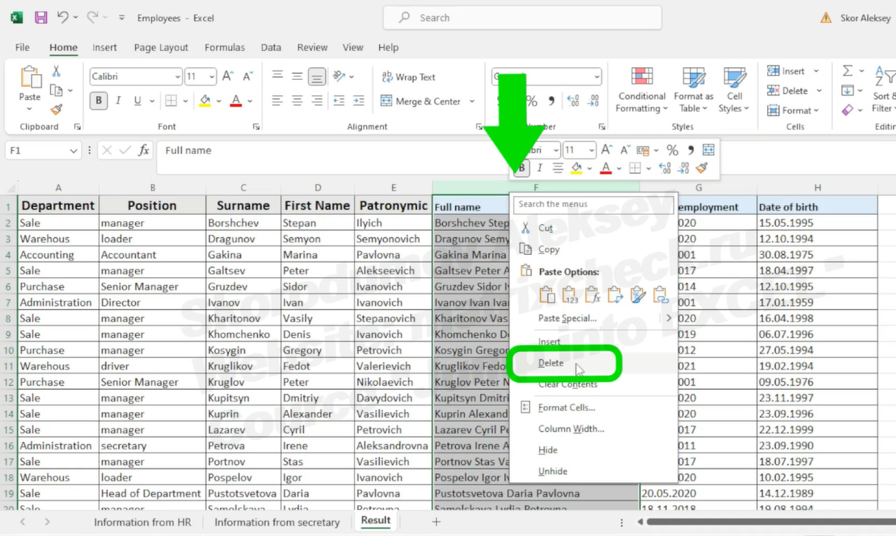
Thus, all the original data has been transferred to the «Result» sheet.

Сreating a new column

Let’s create the columns «Experience of full years on the date of the report» and «Age of full years on the date of the report» ourselves.

To do this, we stand on the cell «H1» and type «Experience of full years on the date of the report». Then we stand on the cell «I1» and type «Age of full years on the date of the report».

In this form, the table is not suitable for printing: the top row of the table with column headers (it is often called a «Table Header row» or just «Header») has a font of different sizes in different columns, as well as different fill.